Methods: Biodiversity Indicators
Summary of methods for defining biodiversity indicators, analyzing data, and summarizing results.
.svg)
As part of interpreting biodiversity indicators, we describe species’ habitat associations. Because the habitat needs of many species are not well known, especially for soil mites, lichens, and mosses, we base many of these associations on ABMI monitoring data. Habitat associations are defined by the vegetation types where species are most abundant. For example, a species is considered associated with older deciduous and mixedwood forests if it is more abundant in these stand types than in other vegetation or human footprint types, and more abundant in older stands than in mid-seral or young stands. These associations may change for some species as more data become available. Habitat associations for all species reported here can be found in the ABMI's Biodiversity Browser.
Biodiversity Intactness
The ABMI collects data on six taxonomic groups (birds, mammals, soil mites, vascular plants, mosses, and lichens) and builds empirical-statistical models to identify how the occurrence and relative abundance of species varies in relation to native land cover, direct human footprint (based on HFI 2023), and spatial/climate variables. For species with sufficient data, we determine cumulative effects of human footprint on habitat suitability for species by comparing predictions under current landscape conditions to predictions in reference landscapes where all human footprint has been removed (the “backfilled” landscape). We convert the difference in habitat suitability between predicted current and reference abundances to a scaled Biodiversity Intactness Index.
The Intactness Index is scaled between 0 and 100, with 100 representing no difference in expected suitability between current and reference conditions, and 0 representing current habitat suitability as different from reference conditions as possible. Intactness thus reveals deviations in habitat suitability from intact conditions. Differences in suitability from reference conditions in either the positive and negative direction are viewed as deviations from intact. For example, an intactness value of 50% means that the current habitat suitability is either half or twice as much as that predicted under reference conditions. The index is calculated as:
- current / reference × 100%, when current < reference (these are "decreaser" species whose relative abundance is lower in human footprint compared to reference conditions), or
- reference / current × 100%, when reference > current (these are "increaser" species whose relative abundance is higher in human footprint compared to reference conditions).
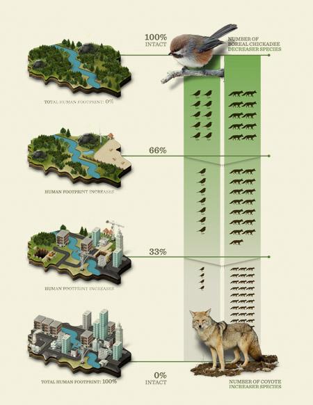
Overall intactness for a region is calculated by averaging intactness of species within each taxonomic group, then averaging the six taxonomic groups. Because increasers and decreasers both reduce intactness, a predicted increase in one species does not cancel out a predicted decrease in another species. Instead, both reduce intactness.
See infographic below for a visual example of how decreaser and increaser species respond to changes in habitat suitability.

To help interpret the species intactness index, we use the following ranges:
- 90–100%: High biodiversity intactness
- 80–90%: Moderately high intactness
- 60–80%: Moderate intactness
- 40–60%: Moderately low intactness
- Below 40%: Low intactness
Values above 90% generally indicate that habitat suitability for biodiversity is in good condition compared to an undisturbed reference landscape, and are described as having “high” intactness for the assessed region. These thresholds are working guidelines and may be refined in future as new information and improved models become available.
See Section 4.1 for biodiversity intactness results.
The Biodiversity Intactness Index is a coarse-scale indicator that summarizes the overall state of biodiversity across many species in a region. However, a single value cannot show that some areas within the region have higher or lower intactness than the regional average. For example, some sites within a region may be nearly 0% intact (e.g., active industrial sites), while others may be close to 100% intact (e.g., undisturbed forest habitat). Mapping the index helps identify where local-scale impacts from more intensive land-use activities are occurring within the region.
Sector Effects
Identifying the species most affected by an industrial sector can help in land use planning and, if necessary, in developing mitigation strategies. However, with several industries operating on the same land base, it can be difficult to distinguish what effect each industry is having on which species. To assess this, the ABMI combines our breadth of species habitat models with land base information to infer the effects of different industrial sectors on species[1,2].
Local Sector Effects
Values of local sector effects indicate how much habitat suitability for a species change in the exact area where a sector’s footprint occurs. It is the difference between the habitat suitability for a species in the native habitat prior to the footprint and habitat suitability for the species directly on the sector’s footprint. Results are interpreted as follows:
- If there is no suitable habitat at all for the species within the sector’s footprint, the local sector effect is -100%.
- If suitable habitat for the species does not change between native habitat and footprint, the effect is 0%.
- If a species prefers footprint, the effect is a positive percentage reflecting the magnitude of increase from native habitat suitability.
Regional Sector Effects
Regional sector effects capture how much the habitat suitability across a given region is predicted to have changed due to that sector’s footprint in that region. It is the difference between the habitat suitability for the species in the reference landscape with all human footprint removed, and the reference landscape with just that sector’s footprint added back in. Three factors determine a sector’s effect on the regional habitat suitability for a species:
- How much area that industry’s footprint occupies. All else being equal, the more area a sector’s footprint occupies, the more effect it will have on habitat.
- The local sector effect of that sector on the species (described above). Habitat suitability for a given species may be reduced in one sector’s footprint, remain the same in another’s, and increase in other footprint.
- The habitat types that the industry operates in. A sector’s effect on the regional habitat suitability for a species will be greater if the industry operates more in good habitat for the species. For example, two forest species might both avoid agricultural areas, but one lives in aspen stands and the other in Black Spruce. Agriculture will have a much greater effect on the regional habitat suitability for the aspen species, because agricultural clearings are often in aspen stands and rarely in Black Spruce.
Species most negatively affected by an industrial sector will therefore be those that are least tolerant of that sector’s footprint and that prefer to live in habitat types where more of the sector’s footprint occurs. People interested in knowing which species are the most affected by an industrial sector—positively or negatively—should look at the regional sector effects.
Step 1. We develop habitat models for species based on ABMI field data.
Step 2. We define six industrial sectors:
- Agriculture: Cultivated crops or pastures. Note that agriculture is not summarized in this report because there is effectively no agriculture in the Al-Pac FMA area.
- Forestry: Age and stand type of harvest areas are tracked to account for recovery.
- Energy: Mines, well sites, pipelines, transmission lines, seismic lines and associated facilities.
- Transportation: All roads and rail lines. We cannot distinguish roads made specifically for other sectors, such as roads to access harvest areas or well sites.
- Urban/Industrial: Residential, industrial or recreational sites in rural or urban areas.
- Miscellaneous (not reported): Includes human-created water and unclassified footprint.
Step 3. Using the habitat models, for each sector separately, we predict habitat suitability for each modelled species both in the reference backfilled landcover map and the reference map plus the sector’s footprint. We use the differences in habitat suitability just in the areas of the sector’s direct footprint to calculate the local sector effect. We use the differences in total abundance over the whole region to calculate the sector’s effect on the regional habitat suitability for the species.
There are two important caveats for the sector effects:
- The results are based on applying our habitat models to land base information. The models have statistical uncertainty, and there may be errors in the land base information. We do not yet have direct field measurements on actual trends in species’ abundances related to different industrial sectors.
- This is a fairly simple approach that does not account for non-footprint effects (e.g., pollution), or complexities like interactions between sectors (e.g., weedy species entering one sector’s footprint after they were introduced by another sector). We also have to use rules to account for areas where different sectors overlap (e.g., a well site in a cultivated field, forest harvest prior to an industrial development).
See Section 4.2 for sector effects results.
Attribution of Species Habitat Change
The ABMI continues to collect data to meet our long-term goal of calculating trends in species’ abundances. However, we currently lack adequate data for most species to calculate observed trends. Until those direct trend estimates are available, we can report trends in species habitat inferred from changes in the land base.
In this report, we used species habitat models to predict species abundance within Al-Pac’s FMA area, using complete maps of native vegetation and human footprint from 2010 and 2023, and report the predicted change in the species over that time. Six causes of change in species abundance between 2010 and 2023 are identified:
- Aging of native forest that is undisturbed over the period,
- Aging of harvest areas that already existed on the land base in 2010,
- Fires that occurred within the period,
- New forestry footprint that was established within the period,
- New non-forestry human footprint, established within the period that replaced native habitat and/or harvest areas, and
- Changes in non-forestry human footprint that already existed on the land base in 2010.
Currently, only undisturbed native vegetation and forestry footprint increases in age within the land base summaries. Other non-forestry human footprint persists in the land base summaries unchanged unless it transitions to a different type of human footprint. Component #6 above is therefore always a relatively small area.
We use “arrow diagrams” to show the effects of each type of land base change on species. To interpret the arrow diagrams, follow the arrows from the top of the figure, starting at 0% change, to the bottom to see the predicted effects on the species of:
- new forestry, then
- the effect of old regenerating harvest areas, then
- new non-forestry human footprint, then
- transitions of old non-forestry human footprint to another footprint type, then
- fires, and finally
- aging of undisturbed native forest.
The endpoint is thus the net change of all effects predicted in that species from 2010 to 2023.
For each taxonomic group we present figures which compare the effects of:
- Forestry: New forestry footprint (harvested between 2010 and 2023), regenerating old forestry footprint (harvested before 2010 and continuing to regenerate), and combined forestry effect.
- Other human footprint: New non-forestry footprint (created between 2010 and 2023), old non-forestry footprint (present before 2010), and net effect of non-forestry footprint.
- All human footprint combined.
- Natural processes, including fire (areas burned between 2010 and 2023), aging of undisturbed stands, and net change from these natural processes.
- All land base changes combined.
- 2023 Fire, including all areas burned in 2023.
We highlight the effects of each type of land base change on species habitat in the Al-Pac FMA area.
- These changes reflect the predicted changes in species due to changes in the land base that we can map. Many other factors can also change species’ populations. We will be able to look into those when we have direct trend information, which we can then compare to the changes predicted from land base change.
- These predicted effects of land base change are based on the period 2010–2023. Harvest rates, and particularly fires, vary over time. The ABMI will soon have province-wide mapping for the year 2000, so that we can extend the attribution analysis over a longer time period.
- The results are based on ABMI habitat models, which are imperfect and improve over time as we collect more data.
- This analysis represents how natural landscape processes and human footprint impact biodiversity across a wide breadth of species for an entire region. Similar to the Biodiversity Intactness Index, this single value does not reflect that there are areas within the region with both higher and lower levels compared to the regional indicator status.
See Section 4.3 for species habitat change results.
Species of Conservation Concern
Al-Pac defines "Species at Risk" (SAR) as federally and/or provincially listed and known or expected to occur within the FMA area based on range maps, records, and expert knowledge. This list is updated annually and includes:
- federally listed as Endangered, Threatened or Special Concern under Canada’s Species at Risk Act (SARA);
- provincially listed as Endangered or Threatened under Alberta’s Wildlife Act;
- recommended for listing federally by the Committee on the Status of Endangered Wildlife in Canada (COSEWIC), or provincially by Alberta’s Endangered Species Conservation Committee (ESCC) as Endangered, Threatened, or Special Concern.
See Section 5.1 for information on species at risk, including status ranks, occurrence information, and biodiversity intactness scores for those species with enough detections.
Occurrence is expressed as the percentage of ABMI sites where a species was detected out of all sites monitored. For sites visited more than once, each species is counted only once to ensure occurrence is based on unique detections.
Note that intactness is a measure of the predicted effects of local human footprint on habitat suitability; it is not a measure of population trend. Further, the ABMI cannot assess the status of all species of conservation concern in Al-Pac's FMA area for one of two reasons. First, by virtue of their rarity, some species of conservation concern were simply not detected or were not detected with enough frequency to adequately assess their status. Second, the ABMI monitoring protocols are not designed to monitor some species groups, such as owls, waterfowl, and bats, that include some species of conservation concern.
Data were collected from 2003 through 2019 for birds and mosses; 2015 through 2021 for mammals; and 2003 through 2021 for lichens and vascular plants.
Non-native Vascular Plants
Occurrence is expressed as the percentage of ABMI sites where a species was detected out of all sites monitored. For sites visited more than once, each species is counted only once to ensure occurrence is based on unique detections.
References
Sólymos, P., E.T. Azeria, D.J. Huggard, M.-C. Roy, J. Schieck. Chapter 4: Predicting Species Status and Relationships. In ABMI 10-Year Science and Program Review, Available at: https://abmi10years.ca/wp-content/uploads/2019/01/ABMI_10-yr_review_v8_Jan_2019.pdf.
Sólymos, P., J. Schieck. 2016. Effects of Industrial Sectors on Species Abundance in Alberta. Available at: https://abmi.ca/publication/437.html.
